Front End

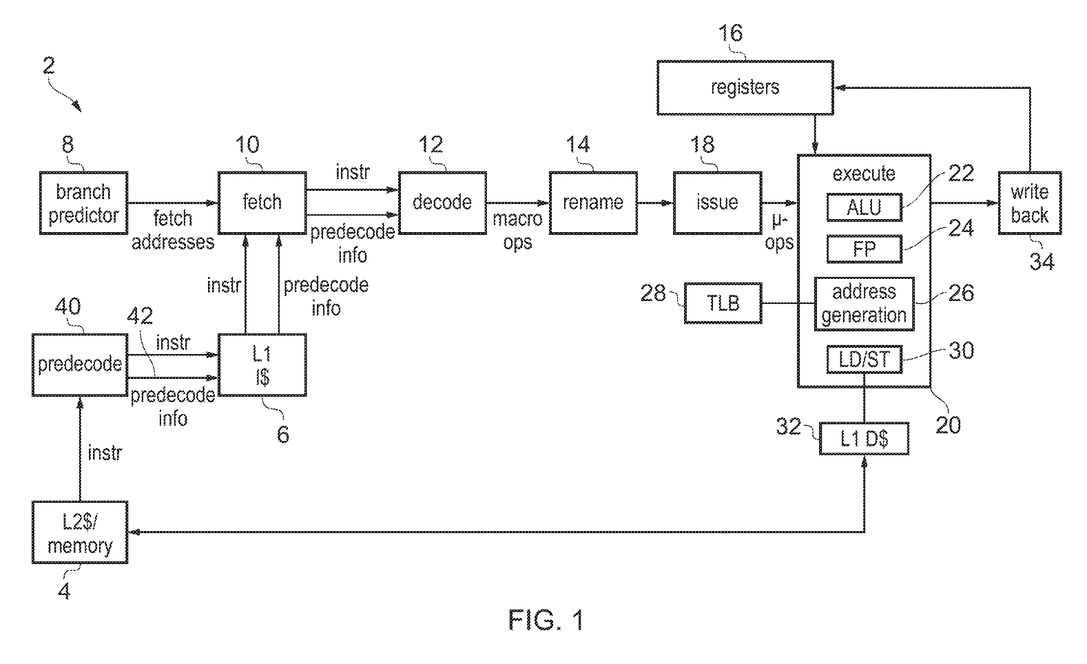
These are the things that happen in-order prior to out-of-order execution.

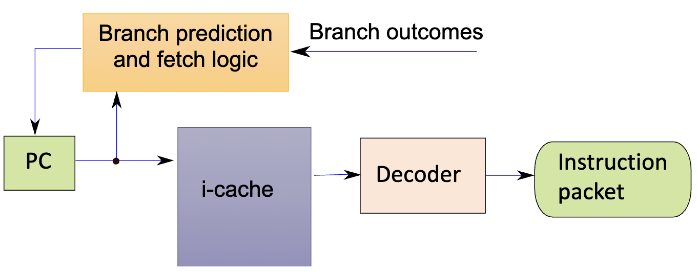
High-Level Architecture of Front End

Branch prediction and fetch logic unit computes address of next instructions to be fetched.

These instructions are fetched from the instruction cache (I$).

Instructions are passed to decoder for turning into instruction packets (sometimes also called “backpacks”).

Instructions and Cache Lines

Assume a fetch width of 4 and cache line size of 64B. Then four consecutive instructions can span up to two consecutive cache lines. But what if some of these instructions are branches? If we can’t fetch the right instructions, we’re just doing extra work for no reason and wasting time and cycles. We could use a better predictor.

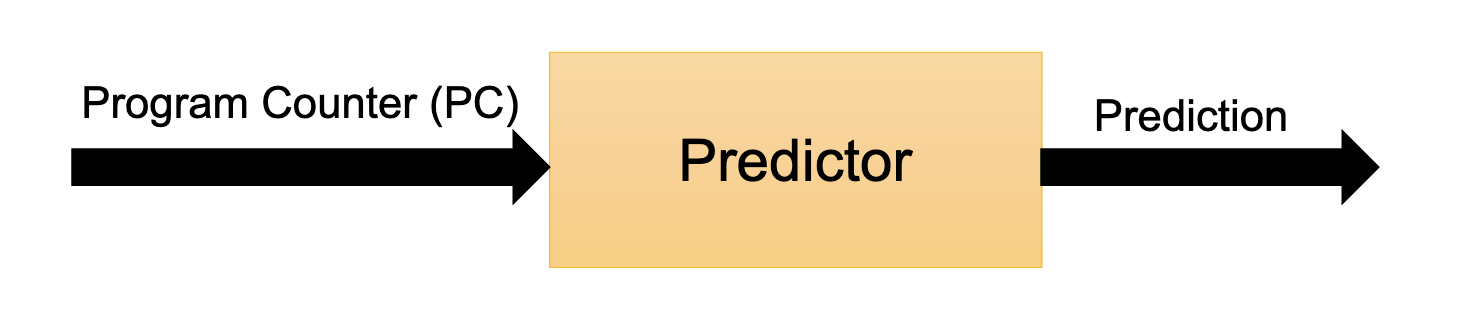
Branch Prediction

Branch Prediction

Problems

In reality, there are three subproblems to this:

• Predicting the instruction type: is this instruction a branch (i.e., can it cause non-sequential control transfer)?
  • Yes: {B, BR, B.cond, BL, BLR, RET}; no: everything else in ISA
• Predicting the branch outcome: If the instruction is a branch, will it be taken or not?
  • Unconditionally taken: {B, BR, BL, BLR, RET}; conditionally taken: {B.cond}
• Predicting the branch target: If the branch is taken, to which non-sequential address will it transfer control?
  • Statically known: {B, BL, B.cond}; dynamic: {BR, BLR, RET}

We need to make relevant predictions based solely on PC value and prior knowledge.

What we want to do is gather information from what happened before.

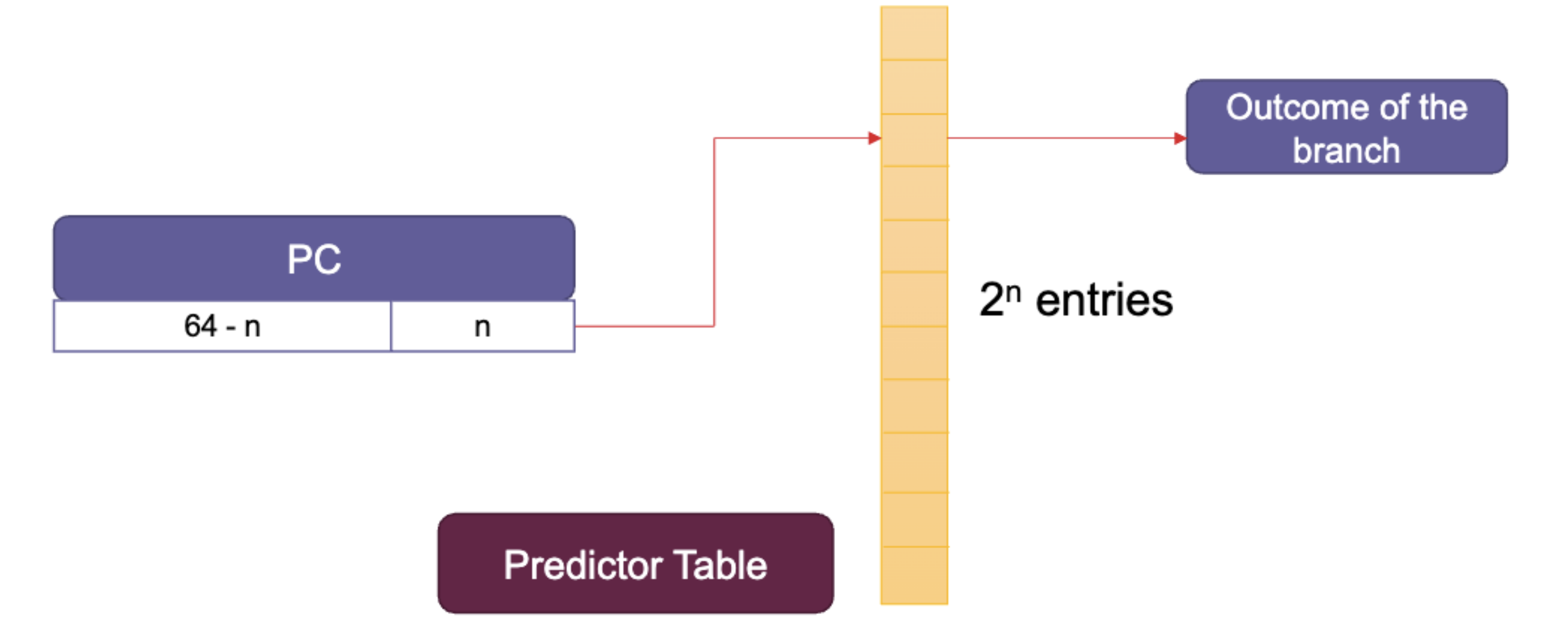
Predicting Instruction Type

Observation: the type of the instruction at a program counter (PC) is static

Implication: maintain a lookup table (the Instruction Status Table, or IST) to record and look up this information.

There are some considerations of this: size of the table, taking advantage of instruction alignment, keeping additional information in IST, aliasing between instructions.

Predicting the Branch Outcome

Imagine we have C code like the following:

void foo() {
	for(int i = 0; i < 5; i++) {
		...
	}
}

Simplified assembly can be described as:

.foo:
	mov r0, 0
.loop:	
	cmp r0, 5
	beq .exit
	add r0, r0, 1
	bne .loop
.exit:
	NOP

The loop is the critical path and most of the time will be predicted not taken. We will use a simple bimodal predictor.

If we use a single-bit predictor, we remember the last outcome, and the current prediction becomes the last outcome.

The misprediction rate is $\frac{1}{6}$ for the first call to foo and $\frac{2}{6}$ for the second and onwards.

Improving Accuracy

We can always add extra bits to the table.

The beq instruction in foo is fundamentally biased towards not taken

• One exception at loop exit shouldn’t impact this tendency significantly
• Add hysteresis

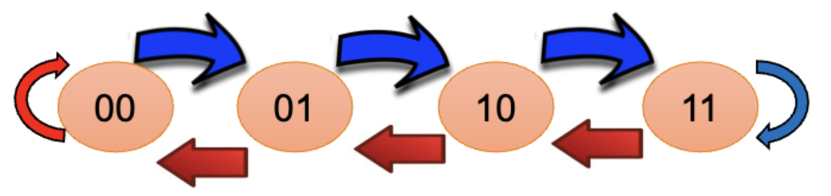
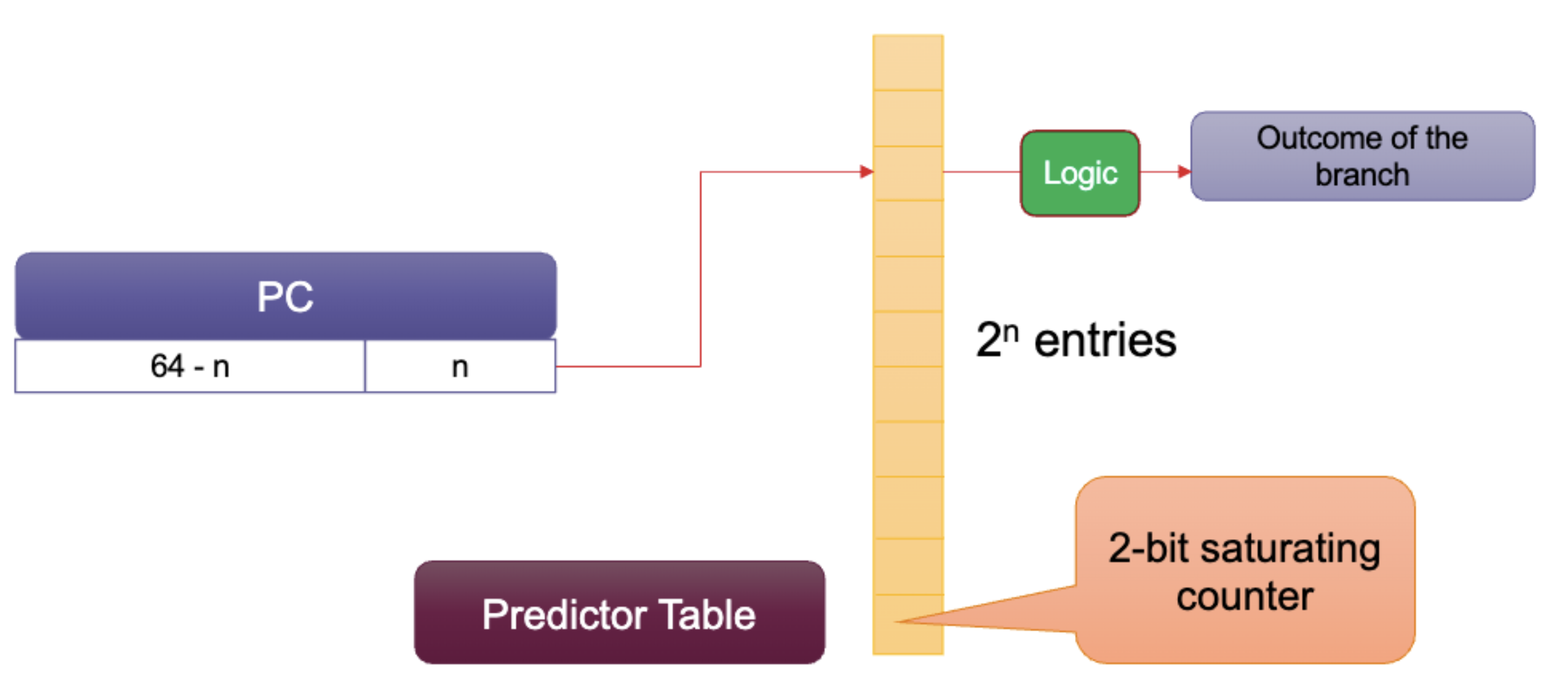
Use a saturating counter, increment when taken, decrement when not taken.

We can predict not taken when we have 00 or 01, and predict taken when we have 10 or 11.

This is a Moore finite state machine. We start from 01 and the misprediction rate eventually decreases to $\frac{1}{6}$.

Global History

We need to have a shift register that records the history of the last $k$ branches encountered by the processor.

We have one bit for each branch, regardless of the PC. We record 1 for branch taken and 0 for branch not taken.

Consider a 2-bit global history register (GHR) like this:

We have two conditional branches in the running example: beq .exit and bne .inc

Use both $k$ bits of the GHR and least-significant $n$ bits of the PC to index into the pattern history table (PHT). The PHT has $2^{n+k}$ entries and increased accuracy.

This is also called a GAp two-level adaptive predictor: G for Global, A for Adaptive, p for per-branch/pc.

Invented by UT professor Yale Patt! Yeh & Patt 1991.

Bits used by different configurations

GAp: $k+w\times 2^k\times 2^n$

GAg: $k+w\times 2^k$

PAg: $k\times 2^n+w\times 2^k$

Leveraging Local and Global Information

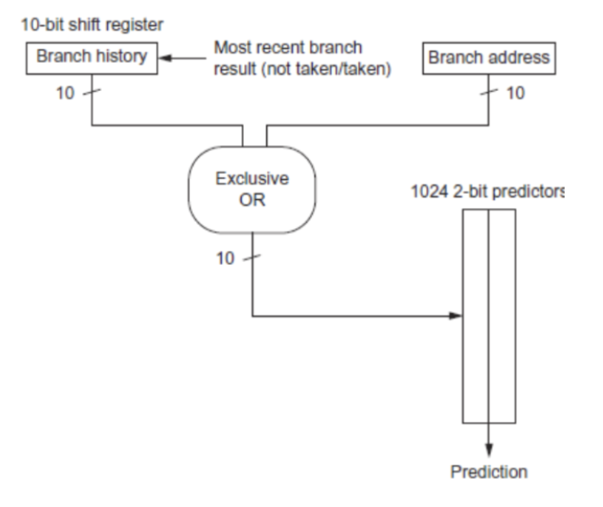
The previous predictors used a ton of data and state to be able to predict branches. We can, however, just use a simple XOR with shared indexes into a prediction table. Eventually, a bunch of addresses and behaviors will converge into a behavior and be placed at a certain index in the table which will then be trained onto local history. Called the “gshare” predictor.

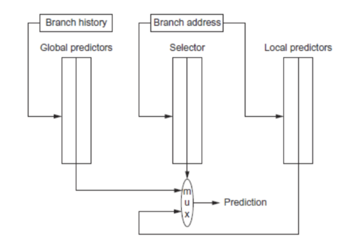
There are also combining or “tournament” predictors used in Alpha 21264.

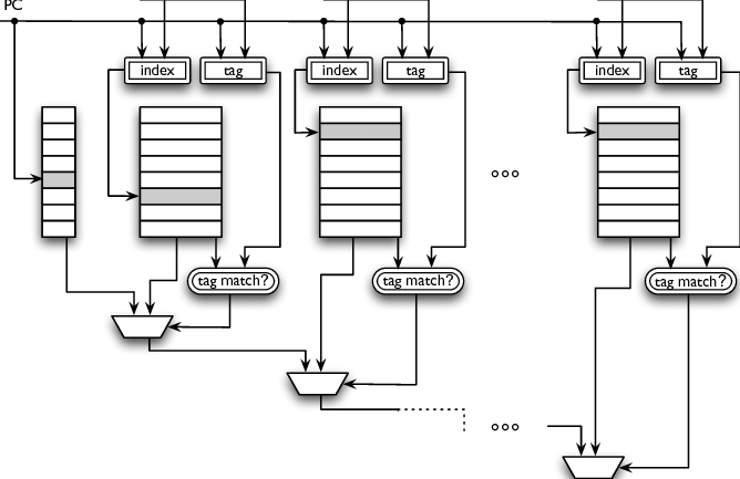
Tagged Hybrid Predictors

Stands for TAgged GEometric predictor (TAGE). It keeps multiple predictions with different history lengths: $L(i)=[a^{i-1}\times L(1)+0.5]$. The hash function can once again just be an XOR. It partially tags predictions to avoid false matches and only provides a prediction on match.

https://www.researchgate.net/figure/The-TAGE-Predictor-with-N-Tagged-Tables-organization-of-the-TAGE-predictor-It-consists_fig1_254023355

Neural Branch Predictor

Invented by UT Student and Professor Calvin Lin! Jiménez & Lin 2002.

The algorithm is to hash the branch address to produce an index $i\in [0,N-1]$ into the table of perceptrons. Fetch perceptron $i$ from the table into a vector register $P_{0:n}$ of weights $\{w_i\}$. Compute $y$ as the dot product of $P$ and the global branch history register (BHR). BHR is encoded as 1 for a branch that is taken and -1 for a branch that is not taken. Predict branch as not taken of $y<0$ and taken otherwise. Once the branch is resolved, use the training algorithm to update the weights in $P$. Write back the updated $P$ into entry $i$ of the table of perceptrons.

The dot product is the slowest/hardest operation so we need to optimize it. To approximate the dot product, we will make the weights $w_i$ small-width integers because we don’t need insane accuracy. Since BHR entries are conceptually $\pm 1$, we just need to add to $w_i$ if it is 1 and subtract if -1. For subtraction we just use $-w_i\approx \overline{w_i}$. Since we only need the sign bit to predict, the other bits can be computed slower.

The training algorithm takes in 3 inputs: $y,t,\theta$ where $t$ is the branch outcome and $\theta$ is a training threshold parameter (hyperparameter). If $\text{sgn}(y)\ne t\text{ or }|y|\le 0$ then forall $i\in [0,n]:w_i\leftarrow w_i+t\cdot x_i$. Empirically, the best threshold $\theta$ for a given history length $h$ is $\theta =\lfloor 1.93h+14\rfloor$.

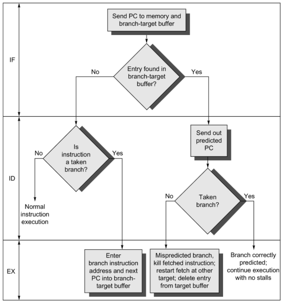
Predicting the Branch Target

Where is the branch target calculated?

• For B, BL, and B.cond, in late Fetch or early Decode stages
• For BLR or RET, in late Decode

This is too late to fetch the correct branch target instruction in the next cycle, even if the prediction is correct, so we need a way of storing the data so we can access it quickly.

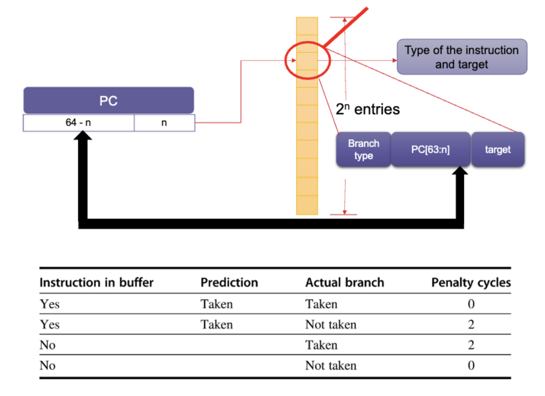
We extend the instruction status table (IST) to keep this information, we call it the Branch Target Buffer (BTB).

The variation is to keep target instructions in the BTB along with (or instead of) the branch target address. This allows branch folding: zero-cycle penalty for unconditional branches (and sometimes for conditional branches as well).

Special Case: Predicting Return Addresses

Since normal call-return protocols are LIFO, use a stack of return addresses to predict branch targets of RET instructions with 100% accuracy (as long as the stack doesn’t overflow). This is called a Return Address Stack (RAS). Push return address when function is called and pop return address when RET is encountered. There are typically 8-16 entries in the stack.

An issue arises, though, how can we handle call depths deeper than this?

We just spill to memory.

A RET is effectively a BR. However, they tell the module whether or not this is a function return within the ISA itself depending on if you used RET or BR, which could be used to add additional details.

Link to original

Decode

Decode

L1 Instruction Memory System

Fetches instruction from the Instruction cache (I$) and delivers the instruction stream to the instruction decode unit.

It includes:

• a 64 KiB (Kibibyte), 4 way Set Associative L1 I$ with 64B lines
• a fully-associative L1 ITLB with native support for 4 KiB, 16 KiB, 64 KiB, and 2 MiB page sizes
• A 1536-entry 4-way skewed associative L0 Macro-Op (MOP) cache, which contains decoded and optimized instructions for higher performance.
• A dynamic branch predictor: TAGe, branch target buffers, return address stacks, etc.

https://www.scs.stanford.edu/~zyedidia/docs/arm/neoverse_v2_trm.pdf

Macro-Ops (MOPs) and Micro-Ops (µops)

Macro-Op (MOP): An instruction held in a format described by the ISA. Can be slight differences, but basically the same. This is independent of the µ-architecture.

Micro-Op (µop): An internal processor specific encoding of the operations used to control execution resources. This can vary widely between different implementations of the same ISA.

The correspondence between MOPs and µops used by a processor may be 1:1, 1:N, or N:1: A single MOP can be cracked/split into one or more internal µops, or multiple MOPs can be fused into a single µop.

Pre-Decoding

https://patents.google.com/patent/US10176104B2/en
The intuition is to identify and signal opportunities to split or fuse instructions into more efficient primitives natively supported by the µarch.

There is, however, a caveat: we need to preserve the precise exception model while doing this.

Examples

Splits

We can split the instruction

str x1, [x2], #24

into the MOP sequence

AGU x2
ALU x2, #24
STR x1

We can split the instruction

stp x29, x30, [sp, #-32]!

into

ALU sp, #-32
AGU sp
STR x29
AGU sp, #8
STR x30

Fuses

We can fuse the instruction sequence

add x0, x1, x2
add x3, x0, x4

into the single MOP

add r3, r1, r2, r4

(assuming the µarch supports 3 register adds)

We can fuse the instruction sequence

b tgt
add x3, x3, 4
tgt: ...

into

nop_pc+8

We can fuse the instruction

cbnz x1, tgt
add x3, x3, 1
tgt: ...

into

ifeqz_add x3, x3, 1, x1, xzr

Instruction Decoding in ARM Cortex-A78

A MOP can be split into two µops after the decode stage. These µops are dispatched to one of 13 issue pipelines where each pipeline can accept 1 µop/cycle.

Dispatch can process up to 6 MOPs/cycle and dispatch up to 12 µops/cycle. There are limitations on each type of µop that may be simultaneously dispatched. If there are more µops available to be dispatched, they will be dispatched in oldest to youngest age-order.

Link to original